Python VTK Sobel 边缘检测:从数学原理到代码实现
本文从图像边缘检测的数学基础出发,完整推导 Sobel 算子的构造过程,并给出 Python + VTK 的可运行实现。文中示意图见 sobel_kernels.svg 与 sobel_vtk_result.svg;本地安装 Python 后运行 sobel_vtk_demo.py 还可导出高分辨率 PNG。


1. 引言
边缘是图像中灰度值发生剧烈变化的区域,例如物体轮廓、纹理突变处。边缘检测的核心问题是:如何在离散像素网格上,稳定地找出“灰度变化最快”的位置?
经典思路来自一阶导数(梯度):
- 灰度变化越剧烈 → 梯度模长越大 → 越可能是边缘。
- 梯度方向 → 边缘的法线方向(垂直于边缘走向)。
Sobel 算子是其中最常用的离散梯度算子之一:它在求导的同时对垂直方向做加权平滑,兼顾边缘响应与抗噪能力。本文将依次讲解:
- 连续梯度与离散差分
- Sobel 核的外积推导
- 3×3 卷积的逐像素展开
- Python VTK 中的
vtkImageSobel2D与vtkImageConvolve实现
2. 一阶导数与二维梯度
2.1 连续情形
设连续图像函数为
f
(
x
,
y
)
f(x, y)
f(x,y),其一阶偏导数描述灰度沿
x
x
x、
y
y
y 方向的变化率:
∇
f
=
(
∂
f
∂
x
,
∂
f
∂
y
)
=
(
f
x
,
f
y
)
\nabla f = \left( \frac{\partial f}{\partial x},\ \frac{\partial f}{\partial y} \right) = (f_x,\ f_y)
∇f=(∂x∂f, ∂y∂f)=(fx, fy)
梯度模长(边缘强度):
∣
∇
f
∣
=
(
∂
f
∂
x
)
2
+
(
∂
f
∂
y
)
2
|\nabla f| = \sqrt{ \left(\frac{\partial f}{\partial x}\right)^2 + \left(\frac{\partial f}{\partial y}\right)^2 }
∣∇f∣=(∂x∂f)2+(∂y∂f)2
梯度方向(边缘方向):
θ
=
arctan
(
∂
f
/
∂
y
∂
f
/
∂
x
)
\theta = \arctan\left( \frac{\partial f/\partial y}{\partial f/\partial x} \right)
θ=arctan(∂f/∂x∂f/∂y)
边缘检测的本质:找出
     ∣

     ∇

     f

     ∣

    $|\nabla f|$

 ∣∇f∣ 较大的像素。
2.2 从变化率到“边缘”
在一维中,
f
′
(
x
)
=
d
f
/
d
x
f'(x) = df/dx
f′(x)=df/dx 表示函数变化快慢。二维图像中,边缘通常对应
∣
∇
f
∣
$|\nabla f|$
∣∇f∣ 的局部极大值。因此,任何实用的边缘算子,最终目标都是估计
f
x
f_x
fx、
f
y
f_y
fy,再合成梯度幅值。
3. 离散差分:像素网格上的导数近似
数字图像是离散采样,不能直接求
    ∂

    f

    /

    ∂

    x

   \partial f/\partial x

∂f/∂x,只能用**差分**近似。
3.1 前向差分
∂
f
∂
x
≈
f
(
x
+
1
,
y
)
−
f
(
x
,
y
)
\frac{\partial f}{\partial x} \approx f(x+1, y) - f(x, y)
∂x∂f≈f(x+1,y)−f(x,y)
实现简单,但不对称,精度较低。
3.2 中心差分(更常用)
∂
f
∂
x
≈
f
(
x
+
1
,
y
)
−
f
(
x
−
1
,
y
)
2
\frac{\partial f}{\partial x} \approx \frac{f(x+1, y) - f(x-1, y)}{2}
∂x∂f≈2f(x+1,y)−f(x−1,y)
∂
f
∂
y
≈
f
(
x
,
y
+
1
)
−
f
(
x
,
y
−
1
)
2
\frac{\partial f}{\partial y} \approx \frac{f(x, y+1) - f(x, y-1)}{2}
∂y∂f≈2f(x,y+1)−f(x,y−1)
中心差分同时利用左右(或上下)邻域,误差阶更高,是 Sobel 等算子的基础。
3.3 差分的卷积核形式
一阶差分可写成极小卷积核:
x 方向:
D
x
=
[
−
1
0
1
]
D_x = \begin{bmatrix} -1 & 0 & 1 \end{bmatrix}
Dx=[−101]
(省略归一化因子
    1

    /

    2

   1/2

1/2 时,仅差一个常数倍,不影响边缘位置。)
y 方向:
D
y
=
[
−
1
0
1
]
D_y = \begin{bmatrix} -1 \\ 0 \\ 1 \end{bmatrix}
Dy=
−101
3.4 简单差分的问题
D
x
D_x
Dx、
D
y
D_y
Dy 只对 3 个像素做运算,**对噪声极其敏感**:单个噪点即可产生虚假“边缘”。Sobel 的改进思路是:**在求导方向保持差分结构,在垂直方向引入平滑**。
4. Sobel 算子的推导:差分 × 平滑(外积)
4.1 设计目标
对 x 方向梯度
G
x
G_x
Gx(检测**垂直边缘**,即灰度沿 x 变化):
| 方向 | 操作 | 作用 |
|---|---|---|
| x | 差分 | 求一阶导数 |
| y | 平滑 | 抑制垂直方向噪声 |
对 y 方向梯度
G
y
G_y
Gy(检测**水平边缘**)则对称:y 方向差分,x 方向平滑。
4.2 基本一维核
x 方向一阶差分:
D
x
=
[
−
1
0
1
]
D_x = \begin{bmatrix} -1 & 0 & 1 \end{bmatrix}
Dx=[−101]
y 方向平滑(三角权重,中心权重更大):
S
y
=
[
1
2
1
]
S_y = \begin{bmatrix} 1 \\ 2 \\ 1 \end{bmatrix}
Sy=
121
平滑核
    [

    1

    ,

    2

    ,

    1

    ]

   [1, 2, 1]

[1,2,1] 可看作小尺度高斯平滑的离散近似,中心像素权重为 2,强调当前行(或列)的信息。
4.3 外积构造
G
x
G_x
Gx
Sobel 的 x 方向 3×3 核由**外积(张量积)**得到:
G
x
=
S
y
⊗
D
x
=
[
1
2
1
]
[
−
1
0
1
]
=
[
−
1
0
1
−
2
0
2
−
1
0
1
]
G_x = S_y \otimes D_x = \begin{bmatrix} 1 \\ 2 \\ 1 \end{bmatrix} \begin{bmatrix} -1 & 0 & 1 \end{bmatrix} = \begin{bmatrix} -1 & 0 & 1 \\ -2 & 0 & 2 \\ -1 & 0 & 1 \end{bmatrix}
Gx=Sy⊗Dx=
121
[−101]=
−1−2−1000121
逐元素计算示例:
第 1 行:
   1

   ×

   [

   −

   1

   ,

   0

   ,

   1

   ]

   =

   [

   −

   1

   ,

   0

   ,

   1

   ]

  1 \times [-1,0,1] = [-1,0,1]
1×[−1,0,1]=[−1,0,1]
第 2 行:
   2

   ×

   [

   −

   1

   ,

   0

   ,

   1

   ]

   =

   [

   −

   2

   ,

   0

   ,

   2

   ]

  2 \times [-1,0,1] = [-2,0,2]
2×[−1,0,1]=[−2,0,2]
第 3 行:
   1

   ×

   [

   −

   1

   ,

   0

   ,

   1

   ]

   =

   [

   −

   1

   ,

   0

   ,

   1

   ]

  1 \times [-1,0,1] = [-1,0,1]
1×[−1,0,1]=[−1,0,1]
4.4 外积构造
G
y
G_y
Gy
y 方向对称地有:
S
x
=
[
1
2
1
]
,
D
y
=
[
−
1
0
1
]
S_x = \begin{bmatrix} 1 & 2 & 1 \end{bmatrix}, \quad D_y = \begin{bmatrix} -1 \\ 0 \\ 1 \end{bmatrix}
Sx=[121],Dy=
−101
G
y
=
S
x
⊗
D
y
=
[
−
1
−
2
−
1
0
0
0
1
2
1
]
G_y = S_x \otimes D_y = \begin{bmatrix} -1 & -2 & -1 \\ 0 & 0 & 0 \\ 1 & 2 & 1 \end{bmatrix}
Gy=Sx⊗Dy=
−101−202−101
即
G
y
=
G
x
⊤
G_y = G_x^\top
Gy=Gx⊤(在标准 Sobel 定义下)。
4.5 示意图
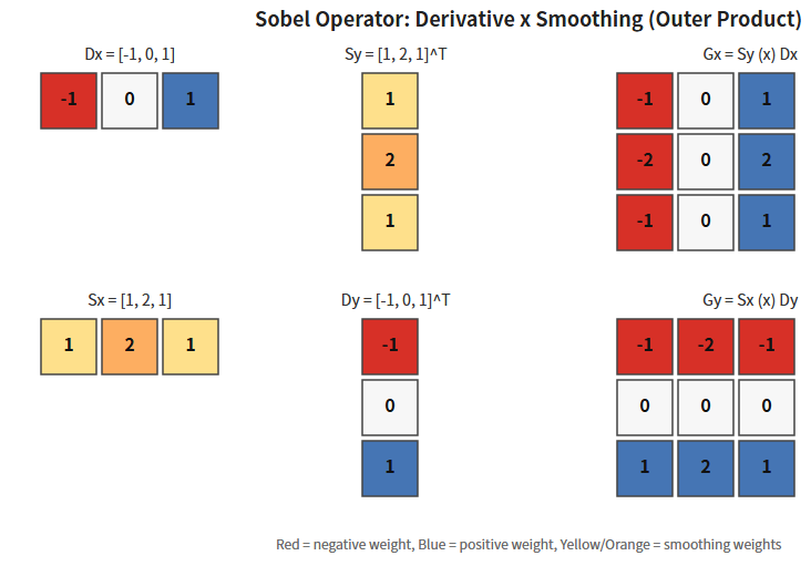
上图直观展示了:
左上:
D x D_xDx 在 x 方向做差分
中上:
S y S_ySy 在 y 方向做加权平均
右上:二者外积得到
G x G_xGx
下行:同理得到
G y G_yGy
5. 3×3 卷积的逐像素展开
设
f
i
,
j
f_{i,j}
fi,j 表示行
i
i
i、列
j
j
j 的灰度(
i
i
i 向下增大,
j
j
j 向右增大),以
(
i
,
j
)
(i,j)
(i,j) 为中心的 3×3 邻域为:
[
f
i
−
1
,
j
−
1
f
i
−
1
,
j
f
i
−
1
,
j
+
1
f
i
,
j
−
1
f
i
,
j
f
i
,
j
+
1
f
i
+
1
,
j
−
1
f
i
+
1
,
j
f
i
+
1
,
j
+
1
]
\begin{bmatrix} f_{i-1,j-1} & f_{i-1,j} & f_{i-1,j+1} \\ f_{i,j-1} & f_{i,j} & f_{i,j+1} \\ f_{i+1,j-1} & f_{i+1,j} & f_{i+1,j+1} \end{bmatrix}
fi−1,j−1fi,j−1fi+1,j−1fi−1,jfi,jfi+1,jfi−1,j+1fi,j+1fi+1,j+1
与
G
x
G_x
Gx 卷积(相关运算,核不翻转):
G
x
(
i
,
j
)
=
(
−
1
)
f
i
−
1
,
j
−
1
+
0
⋅
f
i
−
1
,
j
+
1
⋅
f
i
−
1
,
j
+
1
+
(
−
2
)
f
i
,
j
−
1
+
0
⋅
f
i
,
j
+
2
⋅
f
i
,
j
+
1
+
(
−
1
)
f
i
+
1
,
j
−
1
+
0
⋅
f
i
+
1
,
j
+
1
⋅
f
i
+
1
,
j
+
1
\begin{aligned} G_x(i,j) =\;& (-1)\,f_{i-1,j-1} + 0\cdot f_{i-1,j} + 1\cdot f_{i-1,j+1} \\ &+ (-2)\,f_{i,j-1} + 0\cdot f_{i,j} + 2\cdot f_{i,j+1} \\ &+ (-1)\,f_{i+1,j-1} + 0\cdot f_{i+1,j} + 1\cdot f_{i+1,j+1} \end{aligned}
Gx(i,j)=(−1)fi−1,j−1+0⋅fi−1,j+1⋅fi−1,j+1+(−2)fi,j−1+0⋅fi,j+2⋅fi,j+1+(−1)fi+1,j−1+0⋅fi+1,j+1⋅fi+1,j+1
整理为:
G
x
(
i
,
j
)
=
−
f
i
−
1
,
j
−
1
+
f
i
−
1
,
j
+
1
−
2
f
i
,
j
−
1
+
2
f
i
,
j
+
1
−
f
i
+
1
,
j
−
1
+
f
i
+
1
,
j
+
1
G_x(i,j) = -f_{i-1,j-1} + f_{i-1,j+1} - 2f_{i,j-1} + 2f_{i,j+1} - f_{i+1,j-1} + f_{i+1,j+1}
Gx(i,j)=−fi−1,j−1+fi−1,j+1−2fi,j−1+2fi,j+1−fi+1,j−1+fi+1,j+1
同理:
G
y
(
i
,
j
)
=
−
f
i
−
1
,
j
−
1
−
2
f
i
−
1
,
j
−
f
i
−
1
,
j
+
1
+
f
i
+
1
,
j
−
1
+
2
f
i
+
1
,
j
+
f
i
+
1
,
j
+
1
\begin{aligned} G_y(i,j) =\;& -f_{i-1,j-1} - 2f_{i-1,j} - f_{i-1,j+1} \\ &+ f_{i+1,j-1} + 2f_{i+1,j} + f_{i+1,j+1} \end{aligned}
Gy(i,j)=−fi−1,j−1−2fi−1,j−fi−1,j+1+fi+1,j−1+2fi+1,j+fi+1,j+1
边缘强度:
∣
∇
f
∣
(
i
,
j
)
=
G
x
(
i
,
j
)
2
+
G
y
(
i
,
j
)
2
|\nabla f|(i,j) = \sqrt{ G_x(i,j)^2 + G_y(i,j)^2 }
∣∇f∣(i,j)=Gx(i,j)2+Gy(i,j)2
边缘方向:
θ
(
i
,
j
)
=
arctan
(
G
y
(
i
,
j
)
G
x
(
i
,
j
)
)
\theta(i,j) = \arctan\!\left( \frac{G_y(i,j)}{G_x(i,j)} \right)
θ(i,j)=arctan(Gx(i,j)Gy(i,j))
6. 设计哲学:为何“求导方向差分,垂直方向平滑”?
这是 Sobel 最容易被误解之处,总结为三句话:
- 求导方向必须用差分核,否则无法估计一阶导数。
- 垂直方向必须用平滑核,否则噪声会被差分放大。
- Sobel = 求导方向差分 × 垂直方向平滑(外积)。
6.1 为何 x 方向不能也平滑?
若在 x 方向也使用
    [

    1

    ,

    2

    ,

    1

    ]

   [1, 2, 1]

[1,2,1] 平滑,会把“求导”变成“先平滑再求导”,导致:
- 边缘变宽
- 梯度峰值降低
- 边缘定位不准
Sobel 的设计哲学:求导方向保持敏锐,垂直方向抑制噪声。
6.2 若两个方向都用差分会怎样?
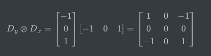
这更接近二阶导数 / Laplacian 型算子,对噪声极度敏感,不是 Sobel 想要的一阶梯度。
6.3 与 Prewitt、Scharr 的对比
| 算子 | 平滑权重 | 特点 |
|---|---|---|
| Sobel |
       [

       1

       ,

       2

       ,

       1

       ]

      [1, 2, 1]

   [1,2,1] | 经典,计算快,工程最常用  |
       [

       1

       ,

       1

       ,

       1

       ]

      [1, 1, 1]

   [1,1,1] | 权重均匀,更平滑、边缘更宽  |
| Scharr | 优化系数 | 更好的旋转不变性,精度更高 |
|---|
Sobel 可理解为“小尺度高斯平滑 + 差分”的 3×3 离散近似。
7. Python VTK 实现
7.1 环境准备
pip install vtk matplotlib numpyVTK 中 Sobel 相关的主要类:
| 类 | 模块 | 作用 |
|---|---|---|
vtkImageSobel2D | vtkImagingGeneral | 内置 Sobel,输出 2 分量梯度向量场 |
vtkImageConvolve | vtkImagingGeneral | 自定义 3×3 核卷积,便于与公式对照 |
vtkImageExtractComponents | vtkImagingCore | 提取 |
G
x
G_x
Gx /
G
y
G_y
Gy 分量 |
| vtkImageMathematics | vtkImagingMath | 计算
G
x
2
+
G
y
2
\sqrt{G_x^2 + G_y^2}
Gx2+Gy2
|
注意:vtkImageSobel2D 的输出是 double 型 2 分量向量场,不是直接的边缘二值图。需提取分量并计算模长,才得到常见的“边缘强度图”。
7.2 方式 A:vtkImageSobel2D(推荐)
# !/usr/bin/env python3
"""Compute Sobel gradients with vtkImageSobel2D."""

import vtkmodules.vtkRenderingOpenGL2  # noqa: F401
from vtkmodules.vtkImagingCore import vtkImageExtractComponents
from vtkmodules.vtkImagingGeneral import vtkImageSobel2D
from vtkmodules.vtkImagingMath import vtkImageMathematics
from vtkmodules.vtkIOImage import vtkPNGReader

def read_grayscale(path: str):
    reader = vtkPNGReader()
    reader.SetFileName(path)
    reader.Update()
    return reader.GetOutput()

def sobel_gradients(image):
    """Return (Gx, Gy, magnitude) as vtkImageData."""
    sobel = vtkImageSobel2D()
    sobel.SetInputData(image)
    sobel.Update()

    extract_x = vtkImageExtractComponents()
    extract_x.SetInputConnection(sobel.GetOutputPort())
    extract_x.SetComponents(0)
    extract_x.Update()

    extract_y = vtkImageExtractComponents()
    extract_y.SetInputConnection(sobel.GetOutputPort())
    extract_y.SetComponents(1)
    extract_y.Update()

    square_x = vtkImageMathematics()
    square_x.SetOperationToMultiply()
    square_x.SetInputConnection(0, extract_x.GetOutputPort())
    square_x.SetInputConnection(1, extract_x.GetOutputPort())
    square_x.Update()

    square_y = vtkImageMathematics()
    square_y.SetOperationToMultiply()
    square_y.SetInputConnection(0, extract_y.GetOutputPort())
    square_y.SetInputConnection(1, extract_y.GetOutputPort())
    square_y.Update()

    sum_sq = vtkImageMathematics()
    sum_sq.SetOperationToAdd()
    sum_sq.SetInputConnection(0, square_x.GetOutputPort())
    sum_sq.SetInputConnection(1, square_y.GetOutputPort())
    sum_sq.Update()

    magnitude = vtkImageMathematics()
    magnitude.SetOperationToSquareRoot()
    magnitude.SetInputConnection(sum_sq.GetOutputPort())
    magnitude.Update()

    return extract_x.GetOutput(), extract_y.GetOutput(), magnitude.GetOutput()
Pipeline 数据流:
7.3 方式 B:vtkImageConvolve 手写 Sobel 核
与第 4 节公式一一对应,适合教学验证:
from vtkmodules.vtkImagingGeneral import vtkImageConvolve

# VTK SetKernel3x3 按行优先排列 9 个元素
GX_KERNEL = [-1, 0, 1, -2, 0, 2, -1, 0, 1]
GY_KERNEL = [-1, -2, -1, 0, 0, 0, 1, 2, 1]

def convolve_sobel(image):
    conv_x = vtkImageConvolve()
    conv_x.SetInputData(image)
    conv_x.SetKernel3x3(GX_KERNEL)
    conv_x.Update()

    conv_y = vtkImageConvolve()
    conv_y.SetInputData(image)
    conv_y.SetKernel3x3(GY_KERNEL)
    conv_y.Update()

    return conv_x.GetOutput(), conv_y.GetOutput()
vtkImageSobel2D 与手写 GX_KERNEL 卷积的结果在数值上应一致(边界处理方式可能略有差异)。
7.4 方式 C:NumPy 对照(无 VTK 时验证公式)
import numpy as np
from scipy.ndimage import convolve

GX = np.array([[-1, 0, 1],
               [-2, 0, 2],
               [-1, 0, 1]], dtype=float)

GY = np.array([[-1, -2, -1],
               [ 0,  0,  0],
               [ 1,  2,  1]], dtype=float)

def sobel_numpy(image: np.ndarray):
    gx = convolve(image, GX, mode="reflect")
    gy = convolve(image, GY, mode="reflect")
    magnitude = np.hypot(gx, gy)
    return gx, gy, magnitude
7.5 完整可运行示例(合成测试图 + 可视化)
同目录 sobel_vtk_demo.py 包含:
- 用 Matplotlib 绘制 Sobel 外积分解图 →
sobel_kernels.png(同目录已附带sobel_kernels.svg示意图) - 用 VTK 在合成图像上运行 Sobel →
sobel_vtk_result.png(同目录已附带sobel_vtk_result.svg示意图)
运行:
python sobel_vtk_demo.py核心 VTK 流程摘录:
from vtkmodules.vtkImagingSources import vtkImageCanvasSource2D
from vtkmodules.vtkImagingGeneral import vtkImageSobel2D, vtkImageConvolve

# 1. 创建测试图(黑底 + 白色矩形 + 圆形)
source = vtkImageCanvasSource2D(extent=(0, 199, 0, 199, 0, 0))
source.SetScalarTypeToUnsignedChar()
source.draw_color = (0, 0, 0)
source.FillBox(0, 199, 0, 199)
source.draw_color = (255, 255, 255)
source.FillBox(40, 80, 40, 160)
source.FillCircle(100, 100, 25)
source.Update()

# 2. Sobel 滤波
sobel = vtkImageSobel2D()
sobel.SetInputConnection(source.GetOutputPort())
sobel.Update()

# 3. 手写核验证
conv_x = vtkImageConvolve()
conv_x.SetInputConnection(source.GetOutputPort())
conv_x.SetKernel3x3([-1, 0, 1, -2, 0, 2, -1, 0, 1])
conv_x.Update()
7.6 运行结果
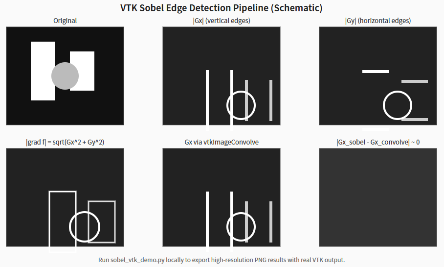
图中可见:
∣
G x ∣ $|G_x|$ ∣Gx∣:垂直边缘(左右灰度突变)响应强∣
G y ∣ $|G_y|$ ∣Gy∣:水平边缘响应强∣
    ∇

    f

    ∣

   $|\nabla f|$

∣∇f∣:综合边缘强度
手写核与
vtkImageSobel2D差异图:接近全零,验证公式与实现一致
8. 工程要点
8.1 输出类型
vtkImageSobel2D→vtkImageData,2 分量 double 向量显示为灰度图前,通常取绝对值并做
vtkImageShiftScale归一化到[ 0 , 255 ] [0, 255][0,255]
8.2 边界处理
卷积在图像边界处缺少完整 3×3 邻域。VTK 各 filter 有默认边界策略;若与 NumPy mode='reflect' 对比,边界若干像素可能存在差异。工程上可:
- 裁剪边界后再分析
- 或预先
vtkImageConstantPad扩展
8.3 从梯度到二值边缘
Sobel 给出边缘强度,若要二值边缘图,还需:
edge
(
i
,
j
)
=
{
1
,
∣
∇
f
∣
(
i
,
j
)
>
T
0
,
otherwise
\text{edge}(i,j) = \begin{cases} 1, & |\nabla f|(i,j) > T \\ 0, & \text{otherwise} \end{cases}
edge(i,j)={1,0,∣∇f∣(i,j)>Totherwise
其中
    T

   T

T 为阈值,常用 Otsu、自适应阈值等方法选取。
9. 总结
| 层次 | 要点 |
|---|---|
| 数学 | 边缘 ≈ 梯度模长极大;离散图像用差分近似导数 |
| Sobel |
G
x
=
S
y
⊗
D
x
G_x = S_y \otimes D_x
Gx=Sy⊗Dx,求导方向差分、垂直方向平滑 |
| 合成 | $ |
|---|---|
| VTK | 生产环境用 vtkImageSobel2D;教学验证用 vtkImageConvolve 手写核 |
三句话回顾:
- 一阶导数 / 梯度是边缘检测的理论基础。
- 离散差分对噪声敏感;Sobel 通过外积引入平滑,更稳定。
- Python VTK 中,
vtkImageSobel2D+vtkImageMathematics即可完整实现 Sobel 梯度与边缘强度计算。